The question I wanted to test
I built a distillation pipeline to investigate a specific question: does a small language model learn differently when its teacher evaluates the responses it actually produces, rather than supplying solutions for it to imitate?
The student was Qwen3-0.6B-Base, with roughly 596 million parameters. The teacher was Qwen3-8B, with roughly 8.19 billion. I implemented the sampling, scoring, training, and evaluation pipeline, then trained LoRA adapters on the student using grade-school mathematics problems from GSM8K. Both models started from existing checkpoints; implementing the process from scratch did not mean pretraining either model.
The most informative result depended on how I asked the trained models to answer. With greedy decoding, which selects the most probable next token at each position, learning from correctness-filtered teacher solutions reached 54.4% test accuracy. On-policy distillation reached 55.0%. That difference alone would give little reason to prefer the more involved procedure.
When I sampled responses instead, the scores were 44.0% and 51.6%. The improvement was 7.6 percentage points on the same 1,319 test problems.
Here, sampled accuracy means mean@4: generate four responses per problem at temperature one, score each, and average their correctness. A problem with one correct response contributes 25%, not 100%. There is no selection of the best answer or majority vote. Temperature one uses the model’s ordinary next-token probabilities, with no top-k or top-p truncation.
The improvement depends on how we decode
The same trained models are almost tied greedily, but separate when their responses are sampled.

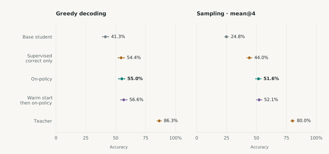
95% interval on the paired difference: +6.10 to +9.10 points. Greedy difference: +0.61 points, with an interval spanning zero.
Read the numerical results
| Model | Greedy | Mean@4 |
|---|---|---|
| Base student | 41.32% [38.82, 44.05] | 24.79% [23.18, 26.52] |
| Supervised correct only | 54.44% [51.93, 57.24] | 43.95% [41.94, 46.10] |
| On-policy | 55.04% [52.31, 57.62] | 51.59% [49.26, 53.77] |
| Warm start then on-policy | 56.63% [54.05, 59.36] | 52.12% [50.02, 54.28] |
| Teacher | 86.28% [84.46, 88.10] | 80.00% [78.49, 81.58] |
Understanding that difference requires some mathematics, but also care about what the experiment actually compared. I will explain the training signal first, then examine the successful runs, a revealing token-level example, and an ablation that made training substantially worse.
What the teacher supplies
From a written answer to a policy
A language model produces a distribution over possible next tokens, the vocabulary units from which its response is assembled. That distribution depends on the prompt and everything it has already written. If the prompt is $x$ and the response so far is $y_{\lt t}$, write the student’s policy as
$$q_\theta(v\mid x,y_{\lt t}).$$Here $v$ is a candidate next token and $\theta$ represents trainable parameters. The prefix is the text before the current token. Changing an earlier arithmetic operation changes the context for every subsequent prediction.
In supervised distillation, the teacher writes a solution and the student learns to make its tokens more probable. At each position, training supplies the teacher-written prefix. This is useful supervision, but it differs from inference, when the student’s own earlier choices determine what it must continue.
A teacher can also supply probabilities. Instead of revealing only its selected token, it reveals how it distributes probability among alternatives. This is the central idea behind the soft targets in Hinton, Vinyals, and Dean’s distillation paper. Probabilities express the teacher’s preferences; they do not certify that those preferences are correct.
What KL divergence measures
For two distributions $p$ and $q$ over the same outcomes, their Kullback–Leibler divergence is
$$D_{\mathrm{KL}}(p\|q)=\sum_v p(v)\log\frac{p(v)}{q(v)}.$$The log-ratio compares the probability assigned to an outcome. The weighting by $p(v)$ then averages those comparisons over outcomes drawn from $p$. We use natural logarithms, giving units of nats.
Consider an illustrative three-outcome vocabulary, with teacher probabilities $p=(0.7,0.2,0.1)$ and student probabilities $q=(0.4,0.4,0.2)$. The contributions to $D_{\mathrm{KL}}(p\|q)$ are approximately $0.392$, $-0.139$, and $-0.069$ nats. Their sum is $0.184$.
The negative contributions are legitimate: on those outcomes the student assigns more probability than the teacher. The total divergence is nevertheless nonnegative, and is zero exactly when the distributions match. Swapping them gives $D_{\mathrm{KL}}(q\|p)\approx0.192$, because both the log-ratio and the weighting change. KL is therefore asymmetric, rather than a geometric distance between distributions.
KL is an average of weighted log-ratios
Some outcomes contribute negatively. The total stays nonnegative, and reversing the comparison changes which distribution weights the average.
1. Compare probabilities
Each model distributes a total probability of 1.
2. Weight each log-ratio
p(v) × log[p(v) / q(v)]
The positive contribution of A exceeds the negative contributions of B and C.
With $p$ denoting the teacher, $D_{\mathrm{KL}}(p\|q)$ is called forward KL and $D_{\mathrm{KL}}(q\|p)$ reverse KL. Forward KL gives substantial weight to outcomes the teacher frequently produces. Reverse KL gives substantial weight to outcomes the student frequently produces, penalizing choices the teacher considers unlikely.
The connection to supervised training is
$$H(p,q)=H(p)+D_{\mathrm{KL}}(p\|q).$$Cross-entropy $H(p,q)=-\sum_v p(v)\log q(v)$ differs from forward KL by the teacher’s entropy $H(p)$, which is fixed during student training. Learning from unfiltered teacher samples estimates a cross-entropy objective. Filtering for correct answers changes the sampled target distribution, and token averaging affects the weighting of variable-length solutions.
Why the total KL cannot be negative
For positive probabilities, $-\log z\geq1-z$. Substituting $z=q(v)/p(v)$ gives
$$D_{\mathrm{KL}}(p\|q)\geq\sum_v p(v)\left(1-\frac{q(v)}{p(v)}\right)=1-1=0.$$Equality requires matching probabilities. More generally, an outcome with positive $p(v)$ but zero $q(v)$ makes the divergence infinite; terms with zero $p(v)$ contribute zero by continuity.
Turning disagreement into a training signal
In on-policy distillation, the student samples a response. The frozen teacher reads that response and evaluates each sampled token using the same prompt and prefix. For teacher policy $p_T$, my implementation assigns
$$r_t=\log p_T(y_t\mid x,y_{\lt t})-\log q_\theta(y_t\mid x,y_{\lt t}).$$A positive reward means the teacher assigns the chosen token more probability than the student does. A negative reward means it assigns less. In the local policy-gradient update, the reward is held fixed while differentiating the student’s log-probability: positive rewards encourage the sampled choice, and negative rewards discourage it. Shared model parameters mean an update also affects other predictions.
At a fixed prefix, averaging over student-sampled tokens gives
$$\mathbb E_{y_t\sim q_\theta}[-r_t]=D_{\mathrm{KL}}(q_\theta\|p_T).$$Thus one negative reward is a sampled estimate of reverse KL, not the exact divergence. It can be negative even though its conditional expectation cannot. The experiment logs both this estimate and the full-vocabulary sum, keeping training feedback distinct from its diagnostic measurement.
For example, suppose the student assigns a token probability 0.2 and the teacher assigns it 0.4. Its reward is $\log(0.4/0.2)=\log 2\approx0.693$ nats. If those probabilities are reversed, the reward is approximately $-0.693$. Neither calculation tells us the total KL: that requires weighting the log-ratio for every possible token. This is why the visualization separates a sampled token’s reward from the distribution-wide measurement.
The two models must also agree on what the outcomes mean. Here they share a tokenizer vocabulary, so a token ID identifies the same text in each distribution. Comparing probabilities at mismatched token IDs would produce a numerical loss without measuring the intended disagreement. The pipeline checks vocabulary alignment before training.
The student writes; the teacher evaluates
The teacher scores each sampled token in the context the student actually produced. Only the student’s parameters are updated.
Teacher writes a solution student learns its next tokens using teacher-written prefixes.
The student writes
Given a prompt, the current student samples a continuation.
q(5 | prefix) = 0.20
The student supplies the prefix.The teacher reads
The teacher evaluates that same token after the same prefix.
p(5 | prefix) = 0.40
Teacher parameters remain frozen.The student learns
The log-ratio supplies a local reward for the sampled token.
log(0.40 / 0.20)
+0.693 natsEncourage this sampled choice.Sample again from the updated student. Its new responses provide the prefixes for the next update.
Step 1: the student samples from its own policy, so training visits prefixes it actually produces.
“On-policy” specifies where the prefixes come from; it does not require a particular KL direction. Agarwal and colleagues explore on-policy distillation with different discrepancy measures. I used a local reverse-KL recipe similar to the one described by Thinking Machines Lab: each token receives its own reward, without accumulating future rewards. This is a practical approximation to the full sequence-gradient formulation. The distinction becomes important in the failed run below.
Constructing the experiment
I used a plain question-and-answer prompt containing four worked examples, identically for teacher and student. That choice followed a failed initial attempt with chat formatting. The base student had not been instruction-tuned for those markers, and its outputs did not reliably terminate in the required format. Training against that baseline could have made learning the response format look like a large improvement in mathematics.
The experiment reserved 500 GSM8K training problems for development, leaving 6,973 training prompts. The standard 1,319-problem test set was evaluated after the development decisions, for the base student, teacher, and three final adapters. All compared results came from one NVIDIA L40S. Answers were extracted using a fixed rule, and responses that exhausted the generation limit counted as wrong.
Mathematics provides a convenient separation between the numerical answer that can be checked automatically and the intermediate explanation that needs closer inspection.
The teacher remained frozen. Student training used rank-32 LoRA adapters on the attention and feed-forward projections. The supervised baseline used 8,000 teacher responses from 2,000 training prompts, with separate runs using all responses or only those whose final answer was correct. Each ran for 400 optimization steps.
On-policy training started from the base student and ran for 300 steps, sampling four responses to each of eight prompts per step. I repeated it with a second training seed. A further run began from the unfiltered supervised adapter and added 200 on-policy steps at a lower learning rate. I will call that the warm-start model.
These settings make the recipes interpretable, but they do not isolate one causal variable. Supervision, prefix source, training-token count, and optimization schedule differ between supervised and on-policy training. Training allowed 256 new tokens per response, while final evaluation allowed 512. The sampled metric uses the same temperature and untruncated token distribution as training, with a different response-length limit.
The implementation makes a further distinction between the text a model reads and the positions it learns to predict. Prompts supply context, but only response tokens contribute to the training loss; padding is masked out. The teacher runs without gradients, and the student alone receives parameter updates. Once trained, the student can answer independently of the teacher. Distillation changes its parameters during training rather than introducing a teacher call into each deployed response.
What improved under sampling
The following numbers all come from the test set. Keeping that split explicit matters: development results include more experimental variants, but cannot be inserted into the same comparison as test measurements.
| Model | Greedy accuracy | Mean@4, temperature 1 |
|---|---|---|
| Base student | 41.3% | 24.8% |
| Correctness-filtered supervised distillation | 54.4% | 44.0% |
| On-policy distillation | 55.0% | 51.6% |
| Unfiltered supervised warm start, then on-policy | 56.6% | 52.1% |
| Teacher | 86.3% | 80.0% |
The on-policy student’s sampled improvement over filtered supervised distillation was 7.64 percentage points. A paired bootstrap over test problems gives a 95% interval of approximately 6.1–9.1 points. The greedy difference was 0.61 points, with an interval of approximately −2.0 to 2.9 points. These intervals describe uncertainty over problems for the recorded models; they do not include the variation we would see from retraining every recipe repeatedly.
The paired comparison uses the same resampled problem IDs for both models, preserving the fact that some problems are difficult for both. It also keeps each problem’s four sampled responses together. Treating those responses as four independent benchmark problems would overstate how much independent evidence the evaluation contains. The interval on the difference is more informative here than judging significance from whether two separate model intervals overlap.
There is a practical reason to retain both decoding measurements. If the application always uses greedy generation, the sampled gain alone does not establish a comparable improvement in that application. If it samples candidate solutions, the probability of an individual successful attempt matters directly. This experiment measures that average success probability at one temperature; it does not establish what happens under other temperatures, answer-selection procedures, or downstream tasks. Reporting both metrics lets the reader connect the finding to a deployment choice without treating either score as a complete description of the model.
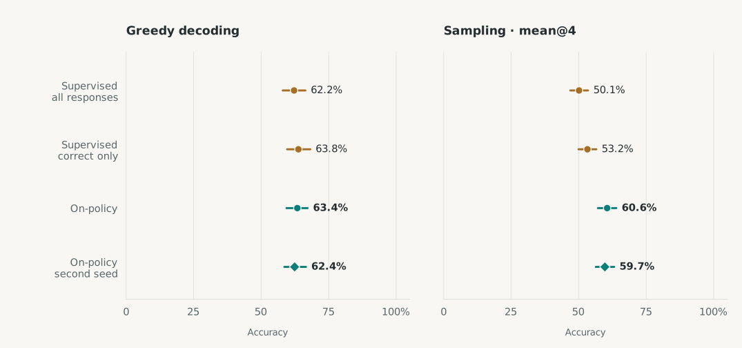
The development runs provide a limited check on that second source of variation. On-policy sampled accuracy was 60.55% and 59.70% across the two seeds, compared with 53.25% for the filtered supervised model. Greedy scores were 63.4% and 62.4%, compared with 63.8%. Both on-policy seeds therefore showed the same qualitative pattern. Two seeds are useful evidence, but not a comprehensive estimate of training variability.
A second seed shows the same pattern
Both on-policy runs improve sampled accuracy over the filtered supervised baseline. Neither improves greedy accuracy in these development measurements.

Read the numerical results
| Model | Greedy | Mean@4 |
|---|---|---|
| Supervised all responses | 62.20% [57.99, 66.40] | 50.15% [46.90, 53.45] |
| Supervised correct only | 63.80% [59.60, 68.20] | 53.25% [49.95, 56.55] |
| On-policy | 63.40% [59.39, 67.20] | 60.55% [57.15, 63.95] |
| On-policy second seed | 62.40% [58.59, 66.60] | 59.70% [56.35, 63.15] |
One expectation had already failed before on-policy training finished. I had thought supervised distillation would contribute relatively little under sampling because it never observes student-generated prefixes. In fact, on development data the unfiltered supervised run increased sampled accuracy from 34.6% to 50.15%, while greedy accuracy rose from 52.4% to 62.2%. Teacher-written solutions improved considerably more than the student’s single most likely response path.
On-policy training added a further improvement under sampling. This is consistent with the motivation for training on contexts the student itself encounters. It does not establish that recovery from an early mistake caused the gain: the recipes differ in other ways, and the direct diagnostic for compounding disagreement was less conclusive than that explanation would suggest.
The warm-start model achieved the highest observed test scores, but its sampled lead over on-policy alone was only 0.53 points. The corresponding interval, approximately −0.9 to 2.0 points, includes zero. It also received additional training. I would treat it as a promising recipe to investigate, rather than evidence that the combined procedure is reliably superior at equal cost.
A correct answer with incorrect intermediate units
Per-token measurements made it possible to inspect something final-answer accuracy does not capture. One development probe asked how many hours it takes to complete 54,000 rope jumps at three jumps per second. The trained on-policy student produced:
54,000 / 3 = 18,000 jumps.
18,000 / 60 = 300 seconds.
300 / 60 = 5 hours.
#### 5
The final answer is correct, but the first intermediate quantity is seconds, and the second is minutes. The arithmetic reaches the right number while the written units describe it incorrectly.
At the position where the student wrote “jumps,” the full-vocabulary reverse KL was approximately 22.7 nats. At “seconds,” it was 8.7 nats. Those two positions account for most of the response’s 42.6 nats of summed divergence. The teacher gave the sampled unit labels very low probability.
Correct arithmetic, incorrect units
At three jumps per second, 54,000 jumps take five hours. The final answer passes, while the teacher strongly disagrees at two intermediate unit labels.
“jumps” · 22.7 nats54,000 ÷ 3 gives seconds.
“seconds” · 8.7 nats18,000 ÷ 60 gives minutes.
The teacher assigns “jumps” much less probability than the student. All values are in nats.
Selection and recorded suffix
Chosen as the correct final-probe response of 30–60 tokens with the largest single-position reverse KL. It is one deliberately selected example, not a frequency estimate. The original response also ends with Question:<|endoftext|>, retained by the known stop-string issue. Downloaded data preserves all 55 tokens. Position indices are zero-based.
This example makes the earlier distinction useful. The reward concerns the token actually sampled. Full-vocabulary KL compares all possible next tokens at that position. A high value locates disagreement between distributions; interpreting it as a semantic error still requires reading the response.
I deliberately selected this example for its large divergence among correct responses of 30–60 tokens. It illustrates what the instrument can reveal, not how common this behavior is. It is also a post-training sample, not a matched before-and-after demonstration that distillation corrected these unit errors.
When future rewards made training worse
The working recipe credited each token with its own reward. I also tried reward-to-go, which credits a token with the sum of its reward and all rewards that follow:
$$R_t=\sum_{s=t}^{T}r_s.$$This has a mathematical motivation. An earlier choice changes the prefixes at which later rewards are obtained, so differentiating the full sequence objective must account for those later consequences. Tests in the repository enumerate a tiny sequence model and verify that the unclipped reward-to-go estimator matches that objective’s gradient. The local estimator does not.
The sequence objective and its gradient
For a fixed prompt and a well-defined distribution over finite responses, write
$$J(\theta)=D_{\mathrm{KL}}(q_\theta(y\mid x)\|p_T(y\mid x))=-\mathbb E_{y\sim q_\theta}\left[\sum_t r_t\right].$$Differentiating the sampling distribution introduces a score-function term. The direct derivative of the log-ratio has zero expectation because $\mathbb E_q[\nabla_\theta\log q_\theta(y)]=0$. Rewards before position $t$ also vanish from its expected score-function contribution, leaving
$$\nabla_\theta J=-\mathbb E\left[\sum_t\nabla_\theta\log q_\theta(y_t\mid x,y_{\lt t})R_t\right].$$Replacing $R_t$ with $r_t$ omits credit for future consequences. It instead gives the local token-KL gradient with the prefix distribution held fixed. This identity describes the idealized estimators; clipping, finite sampling, response truncation, and batch token normalization must be considered separately when interpreting an implementation.
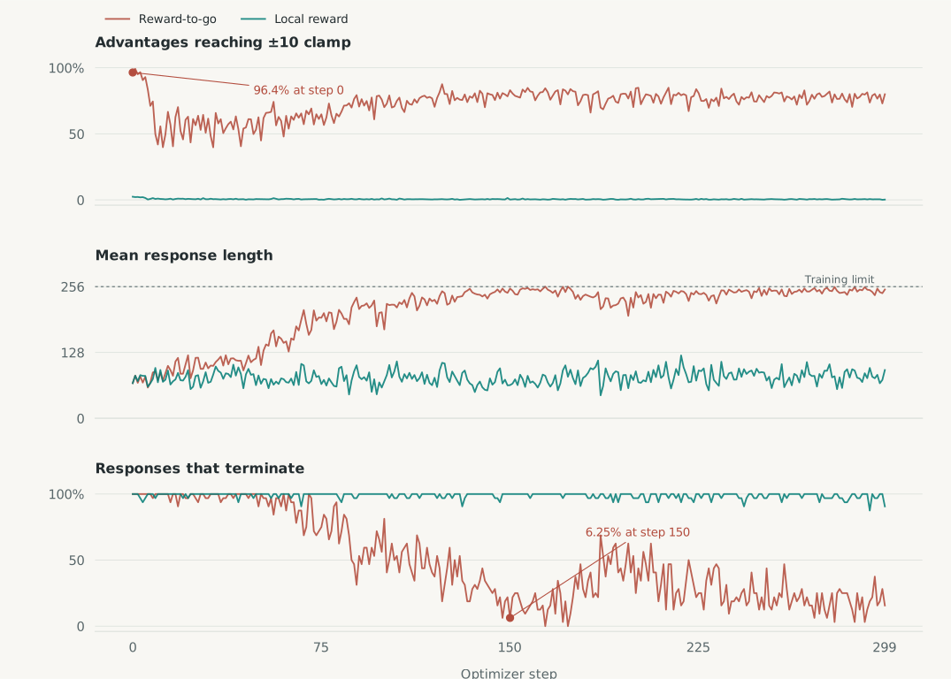
The actual reward-to-go run behaved much worse. At its first step, 96.4% of token advantages reached the implementation’s ±10-nat clamp. Mean training response length grew from about 68 tokens to roughly 250, close to the 256-token limit. By step 150, only about 6% of training responses terminated. The final development sampled accuracy was 45.4%, compared with 60.55% for the local estimator.
Accumulating rewards changed the training dynamics
Reward-to-go saturated the advantage clamp immediately. Longer responses and failing termination followed.

Read the diagnostic checkpoints
| Step | Clamped | Mean length | Terminated |
|---|---|---|---|
| 0 | 96.4% | 68.28 | 100.00% |
| 150 | 83.0% | 252.25 | 6.25% |
| 299 | 80.0% | 250.34 | 15.62% |
The logs suggest why accumulating rewards was problematic here. Expected per-token reward is negative KL. Adding many such rewards can produce large negative returns, especially at earlier positions. Clamping then erases distinctions between returns below −10: very different sequences can receive the same bounded negative signal.
A suitable state-dependent baseline can reduce policy-gradient variance without changing the ideal expected gradient. This run had no learned baseline, and the existing clamp was inherited unchanged from the local recipe. Accumulated negative rewards and saturation are therefore a plausible diagnosis. Demonstrating that a baseline resolves the failure would require another ablation.
The distinction is consequential: the experiment does not show that an unbiased estimator is inherently unusable. It shows a failed training configuration whose clipping substantially changes the estimator, and whose failure becomes understandable only after inspecting more than accuracy or loss.
What the measurements justify
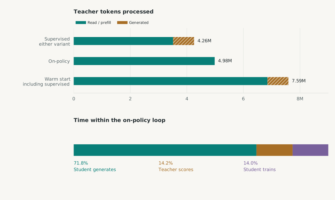
On-policy training changes what work the teacher performs. It scores existing student text in a forward pass instead of generating each response token sequentially. Summed across the main on-policy run, student generation occupied approximately 72% of the measured sampling, scoring, and training time; teacher scoring took about 14%.
That does not establish an end-to-end efficiency advantage over supervised distillation. The supervised recipe processed 4.26 million teacher tokens, including 0.74 million generated tokens. On-policy training processed 4.98 million, all read. The four worked examples added substantial prompt overhead to both. Token counts are not interchangeable with FLOPs or elapsed time, and the supervised data-generation wall clock was not recorded.
Teacher reading and student generation are different costs
The teacher reads more tokens in the on-policy run, while the smaller student spends most of the loop generating responses.

I also tried to test whether disagreement compounded after the first high-KL position. Comparing divergence before and after that crossing initially looked persuasive, until a permutation control exposed the selection effect: everything before the first crossing is below the threshold by construction. Neither on-policy seed exceeded its shuffled comparison; only the warm-start run did. That statistic does not establish recovery from compounding errors as the explanation for the central result.
Nor did held-out KL rank the trained models by accuracy. The warm-start model’s final probe divergence was about 0.602 nats per token, compared with 0.317 for on-policy alone, despite its higher observed accuracy. These measurements use model-dependent sampled prefixes, so they are not comparisons on an identical set of continuations. Even with that qualification, teacher agreement and task correctness remain different quantities.
For this model pair and task, on-policy distillation produced a clear improvement in sampled accuracy over a strong supervised baseline. Greedy evaluation alone would have understated that difference. The next experiments I would prioritize are matched-budget comparisons and a reward-to-go run with an appropriate baseline. Both follow from what these measurements leave unresolved, while preserving the most useful outcome of building the pipeline: a way to examine how the model learns, beyond whether its final answer happens to be right.
Measurement and reproducibility notes
The article uses raw per-question evaluation files, training logs, and token probes from the experiment conducted on 12–13 September 2026. The generated repository summary mixed development and test rows, so it is not the source for these tables. The article’s preparation script checks splits, aligns problem IDs, and recomputes accuracy before producing figure data.
Intervals use 1,000 paired percentile bootstrap resamples over problems, with seed 1234. All four sampled outcomes stay together within each problem. These intervals are conditional on the recorded runs and may differ slightly from the report’s intervals because the bootstrap implementation differs.
The 300-question general-capability probe originally used an unsuitable prompt. Corrected standalone measurements supersede those embedded in older evaluation files. The corrected probe found no clear collapse for the healthy recipes; its size does not establish that specialization has no smaller cost.
Historical training runs lack a recorded source commit. They retain dated run directories and configuration hashes; the later provenance fix cannot reconstruct their missing commits. A known stopping issue also retained trailing text when a stop string occurred before an end token. The excerpt above omits the recorded trailing Question: fragment for readability; the figure data preserves it. These results describe the existing runs, without silently changing their generation or scoring procedure.
Teacher and student sometimes gave the same wrong test answer. That demonstrates agreement on errors, but does not establish that distillation caused a particular error to be inherited. Similarly, solving a question the teacher missed does not identify whether that ability was retained or acquired during training.