Flash Attention: The Mathematical Tricks That Broke the Memory Wall

The Context Length Revolution

In 2022, something fundamental changed in the world of large language models. Suddenly, models that had been stuck processing 2,048 tokens could handle 16,000, then 32,000, then 100,000+ tokens. This wasn’t a gradual improvement—it was a leap forward. The breakthrough that enabled this revolution? Flash Attention, an algorithm that didn’t approximate or simplify attention, but computed it exactly while using radically less memory.

The story of Flash Attention is really a story about understanding your hardware. It’s about realizing that the obvious bottleneck isn’t always the real bottleneck, and that sometimes doing more work can make you faster. Most importantly, it’s about three clever mathematical tricks that, when combined, transform the fundamental scaling characteristics of the Transformer architecture.

The Deceptive Simplicity of Attention

Let’s start with what attention actually computes. At its core, the self-attention mechanism is elegantly simple:

Attention(Q, K, V) = softmax(QK^T / √d) × V

For a sequence of N tokens, each represented by a d-dimensional vector:

• Q, K, V are all N×d matrices
• QK^T produces an N×N attention matrix
• The softmax normalizes each row to sum to 1
• The final multiplication with V produces our N×d output

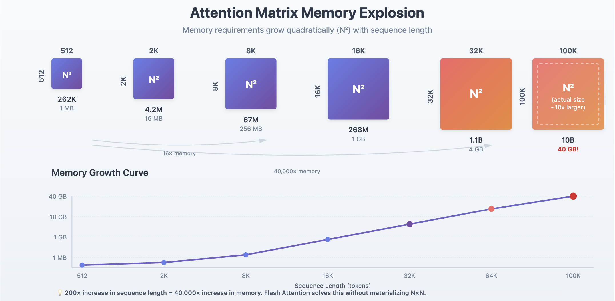
The problem is hiding in plain sight: that N×N attention matrix. When N=2,048, this matrix contains about 4 million elements. When N=16,384, it balloons to 268 million elements. At N=100,000, you’re looking at 10 billion elements—about 40GB in float32. The quadratic growth is devastating.

For years, the research community attacked this problem in the obvious way: try to avoid computing the full N×N matrix. Sparse attention patterns, low-rank approximations, kernel methods—dozens of papers proposed ways to reduce the quadratic complexity. Yet something curious kept happening. These methods would successfully reduce the theoretical FLOP count, but when implemented, they’d often run slower than standard attention.

What was going on?

The Real Bottleneck: A Tale of Two Memories

The answer requires understanding something about modern GPU architecture that’s often overlooked: GPUs have a dramatic memory hierarchy with vastly different performance characteristics at each level.

Consider an NVIDIA A100 GPU:

• High Bandwidth Memory (HBM): 40-80GB of storage, but “only” 1.5-2.0 TB/s of bandwidth
• On-chip SRAM: Just 192KB per streaming multiprocessor, but roughly 19 TB/s of bandwidth

That’s a 10x difference in bandwidth. This massive disparity means that accessing data from HBM is the primary bottleneck in GPU computations. While SRAM can deliver data at blazing speeds, its tiny capacity forces most data to reside in the much slower HBM.

Now here’s the critical insight: standard attention implementations are constantly moving data between HBM and SRAM. They’re not slow because they do too much computation—they’re slow because they spend most of their time waiting for data transfers from the slower HBM memory.

Let’s trace through what standard attention actually does:

1. Load Q and K from HBM → Compute S = QK^T → Store N×N matrix S to HBM
2. Load S from HBM → Compute P = softmax(S) → Store N×N matrix P to HBM
3. Load P and V from HBM → Compute O = PV → Store O to HBM

Each of those loads and stores of N×N matrices is a catastrophic performance hit. The GPU’s computational units, capable of trillions of operations per second, sit idle waiting for memory operations that take orders of magnitude longer than the actual math.

This is why reducing FLOPs didn’t help. The computation was never the bottleneck—memory bandwidth was. It’s like optimizing the mathematical operations when the real problem is the time spent moving data back and forth between memory systems.

Flash Attention’s Three Tricks

Flash Attention solves this memory bottleneck through three interconnected techniques that, together, enable computing exact attention without ever materializing the N×N matrices in HBM. Let’s explore each one.

Trick 1: Tiling — Age Old Divide and Conquer

The first insight is that we don’t need to compute the entire attention matrix at once. Instead, we can break it into small blocks that fit entirely in SRAM.

Think of the attention computation as filling in a giant N×N grid. Standard attention fills the entire grid, then normalizes it, then uses it. Flash Attention says: what if we filled in just one small tile at a time, processed it completely, and then moved on?

The algorithm divides the input sequences into blocks:

• Query blocks of size B_r (typically around √(M/4d) where M is SRAM size)
• Key/Value blocks of size B_c

For each block of the output, Flash Attention:

1. Loads the relevant Q, K, V blocks into SRAM
2. Computes that tile of attention entirely in SRAM
3. Updates the output for that tile
4. Moves to the next tile

The key is that each tile is small enough that all intermediate values stay in the fast SRAM. We never write the full attention matrix to slow HBM.

But wait—there’s a problem. The softmax operation needs to see an entire row to compute the proper normalization. How can we compute softmax correctly when we only see one tile at a time?

Trick 2: Online Softmax — The Mathematical Keystone

This is where Flash Attention’s cleverest innovation comes in: online softmax. This algorithm computes the exact softmax result by maintaining running statistics that can be updated incrementally as we process each tile.

The standard softmax formula for a vector x is:

softmax(x_i) = exp(x_i) / Σ_j exp(x_j)

The online softmax reformulation maintains two running values:

• m: The maximum value seen so far
• l: The sum of exponentials (adjusted for the maximum)

Here’s the magic. When we process a new block of scores, we:

1. Find the new maximum: m_new = max(m_old, max(current_block))
2. Rescale our running sum: l_rescaled = l_old × exp(m_old - m_new)
3. Add the current block’s contribution: l_new = l_rescaled + Σ exp(current_block - m_new)

The rescaling step is crucial—it adjusts previous computations to account for the new maximum, ensuring numerical stability and exactness. When we’ve processed all blocks, we have the exact same result as if we’d computed softmax on the entire row at once.

This isn’t an approximation—it’s mathematically equivalent to standard softmax. The proof relies on the fact that:

exp(x - a) / Σ exp(x - a) = exp(x - b) / Σ exp(x - b)

for any constants a and b. By carefully tracking how our maximum changes and rescaling accordingly, we maintain exactness while never needing the full row in memory.

Trick 3: Recomputation — Trading Compute for Memory

The third trick addresses the backward pass used in training. During backpropagation, we need the attention matrices to compute gradients. Standard implementations store these N×N matrices during the forward pass for use in the backward pass.

Flash Attention takes a radically different approach: it doesn’t store the attention matrices at all. Instead, during the backward pass, it recomputes the pieces it needs on-the-fly.

This seems wasteful—we’re computing the same values twice! But remember: computation is cheap, memory movement is expensive. The time saved by not writing and reading N×N matrices to/from HBM far outweighs the cost of recomputation.

The algorithm stores only:

• The output O (size N×d)
• The softmax normalization statistics (size N)

During backpropagation, when gradients are needed:

1. Reload the relevant Q, K, V blocks
2. Recompute just the attention tiles needed for that gradient
3. Compute gradients entirely in SRAM
4. Accumulate to the final gradient

This is roughly a 2-3x increase in FLOPs, but a 2-4x speedup in wall-clock time. The counterintuitive lesson: in memory-bound operations, doing more work to avoid memory movement is a winning strategy.

Putting It All Together: The Flash Attention Algorithm

Let’s see how these three tricks combine in the actual algorithm. Here’s a simplified view of the Flash Attention forward pass:

Algorithm: Flash Attention Forward Pass
Input: Q, K, V matrices of size N×d
Output: O matrix of size N×d

1. Divide sequences into blocks of size B_r and B_c
2. Initialize output O = 0, running stats m = -∞, l = 0

3. For each K,V block j:
   4. Load K_j, V_j into SRAM
   
   5. For each Q block i:
      6. Load Q_i, current O_i, m_i, l_i into SRAM
      
      7. Compute scores: S_ij = Q_i × K_j^T / √d
      
      8. Update running softmax:
         - m_new = max(m_i, max(S_ij))
         - l_new = exp(m_i - m_new) × l_i + Σ exp(S_ij - m_new)
      
      9. Compute this block's output:
         - P_ij = exp(S_ij - m_new) / l_new
         - O_i = (exp(m_i - m_new) × l_i × O_i + P_ij × V_j) / l_new
      
      10. Store updated O_i, m_i, l_i to HBM

11. Return O

The beauty is in what’s not there: we never materialize the full N×N attention matrix. Each block’s computation happens entirely in SRAM, and we only write back the O(N×d) output.

From Flash Attention to Flash Attention-2

The original Flash Attention was a breakthrough, but it left performance on the table. Profiling showed it achieved only 25-40% of the GPU’s theoretical peak performance. Flash Attention-2 represents a complete algorithmic rewrite that addresses these inefficiencies.

The Parallelism Problem

Flash Attention-1 parallelized across batch size and number of attention heads. But what happens with long sequences and small batch sizes? Many of the GPU’s 108 streaming multiprocessors sit idle.

Flash Attention-2’s solution: also parallelize across the sequence length dimension. Different thread blocks handle different portions of the output sequence, ensuring full GPU utilization even with batch size 1.

The Work Partitioning Revolution

Within each thread block, Flash Attention-1 used a “split-K” scheme:

• K and V were split across 4 warps
• Each warp computed partial results
• Warps had to synchronize and combine results through shared memory

This created a communication bottleneck. Flash Attention-2 flips this to “split-Q”:

• Q is split across warps
• K and V are shared by all warps
• Each warp computes its portion independently with no synchronization

This seemingly simple change eliminates inter-warp communication, reducing shared memory traffic by 4x.

The Results

Flash Attention-2 achieves:

• 50-73% of theoretical peak FLOPS (up from 25-40%)
• 2x speedup over Flash Attention-1
• Up to 9x speedup over PyTorch standard attention
• 225 TFLOPs/s on A100 GPUs for end-to-end training

These aren’t incremental improvements—they’re transformative leaps that make previously impossible model configurations practical.

The Lessons of Flash Attention

Flash Attention teaches us several crucial lessons about algorithm design in the age of specialized hardware:

Profile the Real Bottleneck: The obvious problem (quadratic FLOPs) wasn’t the actual problem (memory bandwidth). Understanding your hardware’s characteristics is essential.

Embrace Hardware Constraints: Rather than fighting the small SRAM size, Flash Attention designs around it. Constraints can inspire innovation.

Exact Beats Approximate: While the research community pursued approximations, Flash Attention showed that exact computation could be faster through better algorithm design.

Recomputation Can Be Free: In memory-bound regimes, trading computation for memory movement is often profitable, a counterintuitive insight that challenges conventional optimization wisdom.

Conclusion

Flash Attention isn’t just a faster attention implementation, it’s a masterclass in hardware-aware algorithm design. By recognizing that memory movement, not computation, was the true bottleneck, and by developing three mathematical techniques to minimize that movement, Flash Attention transformed what’s possible with Transformer models.

The online softmax algorithm, in particular, stands as a brilliant example of mathematical reformulation enabling practical breakthroughs. It shows that sometimes the path forward isn’t to approximate or simplify, but to find clever exact reformulations that align with hardware constraints.

As we push toward ever-longer context windows and larger models, the principles behind Flash Attention—tiling for locality, online algorithms for incremental processing, and strategic recomputation will remain relevant. They remind us that in the modern era of AI, the best algorithms aren’t just mathematically elegant; they’re architecturally aware.

The success of Flash Attention also highlights a broader truth: breakthrough performance improvements often come from questioning assumptions. Everyone “knew” that attention was compute-bound. Everyone “knew” that storing intermediate values was better than recomputing them. Flash Attention proved everyone wrong, and in doing so, enabled the current generation of long-context language models that are transforming AI applications.

The memory wall that seemed insurmountable in 2021 has been broken. Not by approximation, not by new hardware, but by three mathematical tricks and a deep understanding of the machine.

References

1. Dao, T., Fu, D. Y., Ermon, S., Rudra, A., & Ré, C. (2022). FlashAttention: Fast and Memory-Efficient Exact Attention with IO-Awareness. arXiv preprint arXiv:2205.14135.

   • The original Flash Attention paper that introduced the tiling and online softmax algorithms.

2. Dao, T. (2023). FlashAttention-2: Faster Attention with Better Parallelism and Work Partitioning. arXiv preprint arXiv:2307.08691.

   • The follow-up paper detailing the algorithmic improvements in Flash Attention-2.

3. Vaswani, A., Shazeer, N., Parmar, N., Uszkoreit, J., Jones, L., Gomez, A. N., … & Polosukhin, I. (2017). Attention is All You Need. Advances in neural information processing systems, 30.

   • The foundational Transformer paper that introduced the self-attention mechanism.

4. Rabe, M. N., & Staats, C. (2021). Self-attention Does Not Need O(n²) Memory. arXiv preprint arXiv:2112.05682.

   • Important theoretical work on memory-efficient attention computation that influenced Flash Attention’s development.

5. Milakov, M., & Gimelshein, N. (2018). Online normalizer calculation for softmax. arXiv preprint arXiv:1805.02867.

   • Mathematical foundation for the online softmax algorithm used in Flash Attention.

6. Child, R., Gray, S., Radford, A., & Sutskever, I. (2019). Generating Long Sequences with Sparse Transformers. arXiv preprint arXiv:1904.10509.

   • Representative work on sparse attention that, despite reducing FLOPs, often failed to deliver wall-clock speedups.

7. NVIDIA. (2020). NVIDIA A100 Tensor Core GPU Architecture. NVIDIA Corporation.

   • Technical specifications of the A100 GPU architecture that Flash Attention was optimized for.